Time complexity measures the amount of computational time an algorithm takes relative to input size, often expressed using Big O notation like O(n) or O(log n). Space complexity quantifies the memory consumption an algorithm requires during execution to store variables, data structures, and function calls. Explore the nuances of time complexity versus space complexity to optimize algorithm performance effectively.
Main Difference
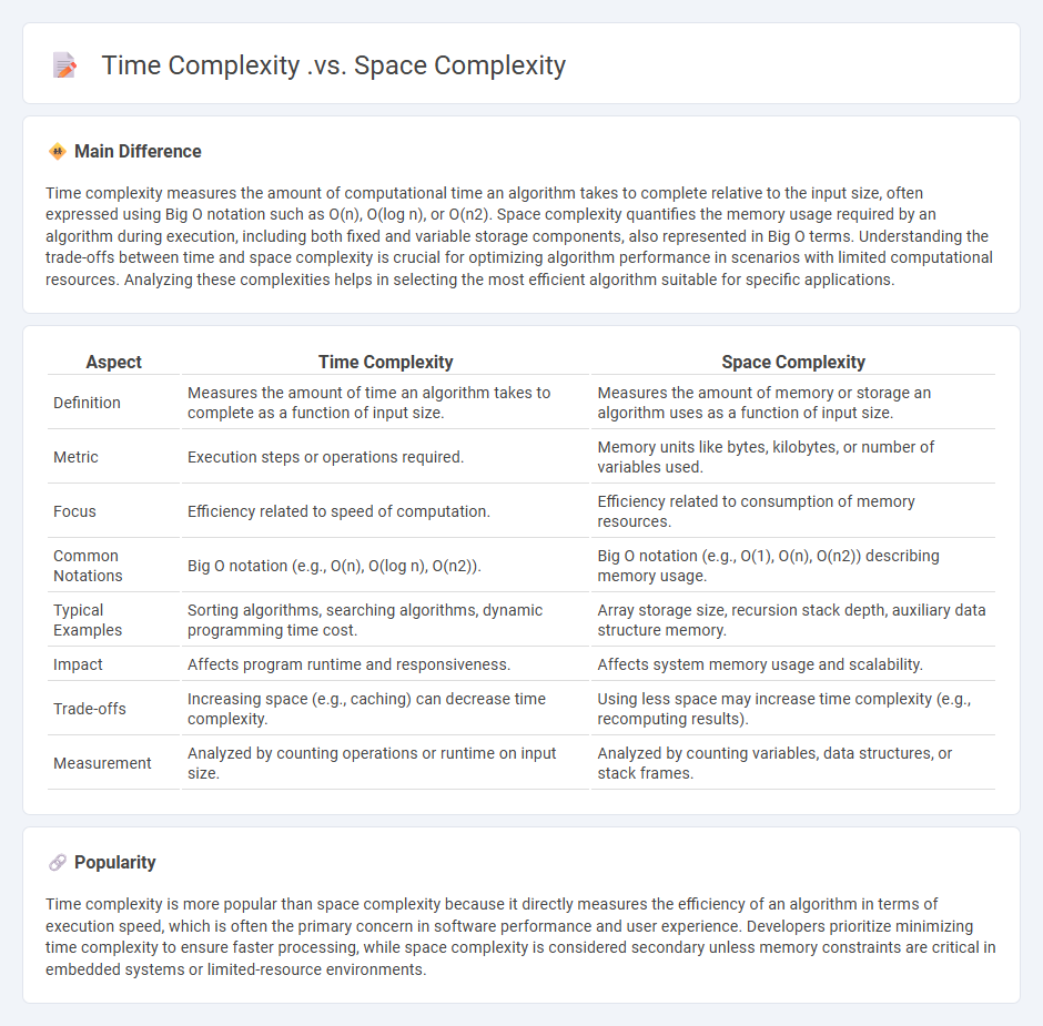
Time complexity measures the amount of computational time an algorithm takes to complete relative to the input size, often expressed using Big O notation such as O(n), O(log n), or O(n2). Space complexity quantifies the memory usage required by an algorithm during execution, including both fixed and variable storage components, also represented in Big O terms. Understanding the trade-offs between time and space complexity is crucial for optimizing algorithm performance in scenarios with limited computational resources. Analyzing these complexities helps in selecting the most efficient algorithm suitable for specific applications.
Connection
Time complexity and space complexity are interconnected metrics that evaluate an algorithm's efficiency by measuring the amount of computational time and memory required, respectively. Algorithms with high time complexity often demand increased space complexity due to the need for storing intermediate computations, while those optimized for lower space usage may trade off with longer runtimes. Understanding this trade-off is essential for designing balanced solutions that optimize both execution speed and memory utilization.
Comparison Table
| Aspect | Time Complexity | Space Complexity |
|---|---|---|
| Definition | Measures the amount of time an algorithm takes to complete as a function of input size. | Measures the amount of memory or storage an algorithm uses as a function of input size. |
| Metric | Execution steps or operations required. | Memory units like bytes, kilobytes, or number of variables used. |
| Focus | Efficiency related to speed of computation. | Efficiency related to consumption of memory resources. |
| Common Notations | Big O notation (e.g., O(n), O(log n), O(n2)). | Big O notation (e.g., O(1), O(n), O(n2)) describing memory usage. |
| Typical Examples | Sorting algorithms, searching algorithms, dynamic programming time cost. | Array storage size, recursion stack depth, auxiliary data structure memory. |
| Impact | Affects program runtime and responsiveness. | Affects system memory usage and scalability. |
| Trade-offs | Increasing space (e.g., caching) can decrease time complexity. | Using less space may increase time complexity (e.g., recomputing results). |
| Measurement | Analyzed by counting operations or runtime on input size. | Analyzed by counting variables, data structures, or stack frames. |
Algorithm Efficiency
Algorithm efficiency measures the performance of an algorithm in terms of time complexity and space complexity, crucial for optimizing computing resources in computer science. Big O notation is commonly used to express the upper bound of an algorithm's running time or memory usage, aiding in the comparison of different algorithms. Efficient algorithms reduce processing time and resource consumption, enhancing software performance in applications like data processing, machine learning, and real-time systems. Advances in algorithm design directly impact computational capabilities in industries ranging from finance to artificial intelligence.
Resource Utilization
Resource utilization in computers refers to the efficient use of hardware and software components such as CPU, memory, storage, and network bandwidth to maximize system performance. Effective resource management techniques include load balancing, process scheduling, and memory allocation, which help prevent bottlenecks and downtime. Modern operating systems monitor resource consumption and dynamically allocate resources based on workload demands to optimize throughput. Advanced metrics like CPU utilization rate, memory usage percentage, and disk I/O operations per second (IOPS) provide insights for performance tuning and capacity planning.
Scalability
Scalability in computer systems refers to the ability to handle increasing workloads or expand resources without compromising performance. It encompasses vertical scaling, which involves upgrading hardware components like CPUs or memory, and horizontal scaling, adding more machines to distribute tasks efficiently. Cloud computing platforms such as AWS and Microsoft Azure provide scalable infrastructure options to manage dynamic demand. Effective scalability ensures systems maintain responsiveness and reliability during peak usage periods.
Computation Speed
Computation speed in computers is primarily measured using clock speed, typically denoted in gigahertz (GHz), with modern processors achieving speeds above 5 GHz. This metric indicates how many cycles per second the CPU can execute, directly impacting the processing power and efficiency of computing tasks. Advances in semiconductor technology and architecture, such as multi-core processors and parallel processing, significantly enhance overall computational speed beyond raw clock rates. Benchmark tests like SPEC CPU and Linpack provide standardized measures of actual performance across different computing systems.
Memory Consumption
Memory consumption in computers refers to the amount of RAM utilized by applications and system processes during operation. Efficient memory management ensures faster data access, improved multitasking, and reduced latency. Modern operating systems, such as Windows 11 or macOS Ventura, incorporate sophisticated algorithms to optimize memory allocation dynamically. Excessive memory consumption can lead to system slowdowns and increased usage of virtual memory, impacting overall performance.
Source and External Links
### 1. Time Complexity vs Space Complexity DifferenceDifference Between Time Complexity and Space Complexity - This article explains how time complexity focuses on execution time relative to input size, while space complexity measures memory usage relative to input size.
### 2. Time and Space Complexity in Data StructuresTime and Space Complexity in Data Structures Explained - This tutorial discusses how time complexity calculates the time required for all statements, while space complexity estimates the memory needed for variables and data.
### 3. Time Complexity and Space Complexity AnalysisTime Complexity and Space Complexity - This article details how time complexity measures the algorithm's execution time as a function of input length, while space complexity quantifies the memory usage as a function of input size.
FAQs
What is time complexity in algorithms?
Time complexity in algorithms measures the amount of computational time an algorithm takes to complete as a function of the input size, often expressed using Big O notation like O(n), O(log n), or O(n^2).
What is space complexity in algorithms?
Space complexity in algorithms measures the total amount of memory or storage space required by an algorithm relative to the input size during its execution.
How do time complexity and space complexity differ?
Time complexity measures the amount of computational time an algorithm takes as a function of input size, while space complexity measures the amount of memory or storage an algorithm requires as a function of input size.
Why is it important to consider both time and space complexity?
Considering both time and space complexity ensures efficient algorithm performance by minimizing execution time and memory usage, which is crucial for scalability and resource-constrained environments.
What factors affect time complexity?
Algorithm design, input size, data structures used, computer architecture, and implementation details affect time complexity.
What factors influence space complexity?
Space complexity is influenced by input size, auxiliary data structures, recursion depth, and variables used during computation.
How can an algorithm be optimized for time and space efficiency?
An algorithm can be optimized for time and space efficiency by using optimal data structures, minimizing redundant calculations through techniques like memoization or dynamic programming, employing in-place computations to save memory, reducing algorithmic complexity (e.g., from O(n2) to O(n log n)), and choosing appropriate sorting or searching methods tailored to the data characteristics.