Fourier Transform decomposes a function into its constituent frequencies, primarily used for analyzing signals in the frequency domain. Laplace Transform extends this concept by converting time-domain functions into complex frequency domains, facilitating the solution of differential equations and system stability analysis. Explore the distinct applications and advantages of Fourier and Laplace Transforms to deepen your understanding.
Main Difference
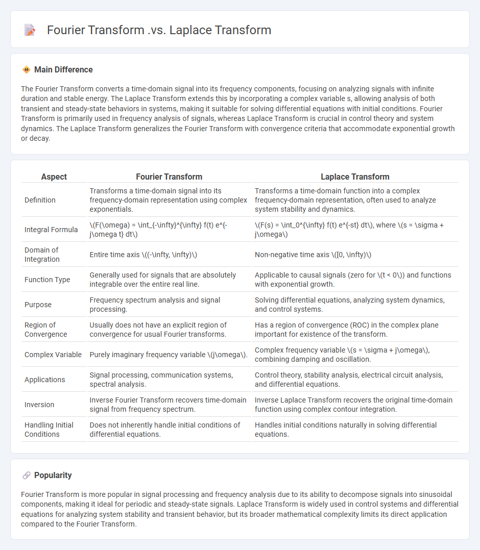
The Fourier Transform converts a time-domain signal into its frequency components, focusing on analyzing signals with infinite duration and stable energy. The Laplace Transform extends this by incorporating a complex variable s, allowing analysis of both transient and steady-state behaviors in systems, making it suitable for solving differential equations with initial conditions. Fourier Transform is primarily used in frequency analysis of signals, whereas Laplace Transform is crucial in control theory and system dynamics. The Laplace Transform generalizes the Fourier Transform with convergence criteria that accommodate exponential growth or decay.
Connection
Fourier Transform is a special case of the Laplace Transform evaluated along the imaginary axis in the complex plane, where the real part of the complex frequency variable is zero. Both transforms convert time-domain signals into frequency-domain representations for analyzing system behavior and solving differential equations. While the Laplace Transform handles a broader class of functions with exponential growth or decay by considering the complex \( s = \sigma + j\omega \), the Fourier Transform focuses on steady-state sinusoidal components with purely imaginary frequency \( j\omega \).
Comparison Table
| Aspect | Fourier Transform | Laplace Transform |
|---|---|---|
| Definition | Transforms a time-domain signal into its frequency-domain representation using complex exponentials. | Transforms a time-domain function into a complex frequency-domain representation, often used to analyze system stability and dynamics. |
| Integral Formula | \(F(\omega) = \int_{-\infty}^{\infty} f(t) e^{-j\omega t} dt\) | \(F(s) = \int_0^{\infty} f(t) e^{-st} dt\), where \(s = \sigma + j\omega\) |
| Domain of Integration | Entire time axis \((-\infty, \infty)\) | Non-negative time axis \([0, \infty)\) |
| Function Type | Generally used for signals that are absolutely integrable over the entire real line. | Applicable to causal signals (zero for \(t < 0\)) and functions with exponential growth. |
| Purpose | Frequency spectrum analysis and signal processing. | Solving differential equations, analyzing system dynamics, and control systems. |
| Region of Convergence | Usually does not have an explicit region of convergence for usual Fourier transforms. | Has a region of convergence (ROC) in the complex plane important for existence of the transform. |
| Complex Variable | Purely imaginary frequency variable \(j\omega\). | Complex frequency variable \(s = \sigma + j\omega\), combining damping and oscillation. |
| Applications | Signal processing, communication systems, spectral analysis. | Control theory, stability analysis, electrical circuit analysis, and differential equations. |
| Inversion | Inverse Fourier Transform recovers time-domain signal from frequency spectrum. | Inverse Laplace Transform recovers the original time-domain function using complex contour integration. |
| Handling Initial Conditions | Does not inherently handle initial conditions of differential equations. | Handles initial conditions naturally in solving differential equations. |
Frequency Domain Analysis
Frequency domain analysis is a critical technique in engineering used to examine signals, systems, and processes by representing them as functions of frequency rather than time. This method is essential for analyzing steady-state responses, filtering, and system stability in electrical, mechanical, and control systems engineering. Tools such as the Fourier Transform, Laplace Transform, and Bode plots enable engineers to identify dominant frequency components and resonance phenomena effectively. Applications include signal processing, vibration analysis, and telecommunications, where frequency domain insights enhance system design and performance optimization.
Time-Domain to Frequency-Domain Conversion
Time-domain to frequency-domain conversion is essential in engineering for analyzing signals and systems. Fourier transform techniques, including the Fast Fourier Transform (FFT), enable efficient decomposition of time-based data into frequency components. This conversion facilitates spectrum analysis, filter design, and system identification in fields such as communications, control systems, and signal processing. Practical applications often involve digital signal processors (DSPs) and software tools like MATLAB for accurate and real-time frequency analysis.
Transient vs Steady-State Response
Transient response in engineering refers to the system's immediate reaction to a change in input or initial conditions, characterized by rapid fluctuations and adjustments before settling. Steady-state response occurs once the system's output stabilizes, maintaining consistent behavior over time despite ongoing inputs. Analyzing both transient and steady-state responses is crucial for designing control systems, ensuring stability, accuracy, and desired performance under dynamic conditions. Key parameters include rise time, settling time for transient analysis, and steady-state error for long-term behavior assessment.
Signal Processing Applications
Signal processing applications span numerous engineering fields including telecommunications, biomedical engineering, and control systems. Techniques such as Fourier analysis, digital filtering, and adaptive signal processing enable efficient data extraction and noise reduction in audio, image, and sensor signals. Real-time processing capabilities support critical functions in radar, speech recognition, and wireless communication technologies. Advances in machine learning integration have further enhanced signal interpretation and anomaly detection accuracy.
System Stability Analysis
System stability analysis in engineering involves evaluating the ability of a system to maintain equilibrium under varying conditions. Techniques such as Lyapunov methods, root locus, and Bode plots are commonly used to assess dynamic stability in control systems. Stability criteria like Routh-Hurwitz and Nyquist provide mathematical frameworks for determining system response to disturbances. Accurate stability analysis is essential for designing reliable systems in aerospace, electrical grids, and mechanical control applications.
Source and External Links
Difference between Laplace Transform and Fourier Transform - The Laplace transform generalizes the Fourier transform with a complex frequency (s-domain) and is suitable for analyzing both stable and unstable systems, while the Fourier transform is confined to real frequency and absolutely integrable functions only.
Laplace transform - Wikipedia - The Laplace transform is defined for functions with suitable decay and allows complex analysis techniques, whereas the Fourier transform decomposes a function into its frequency components but does not have a region of convergence in the complex plane.
Why are the Fourier Transform and Laplace Transform Similar? - The Laplace and Fourier transforms have similar integral forms, but the Laplace transform can be seen as a generalized version of the Fourier transform, with the Fourier transform being a special case when the Laplace variable \(s\) is purely imaginary (\(s = i\omega\)).
FAQs
What is a Fourier Transform?
A Fourier Transform is a mathematical technique that decomposes a function or signal into its constituent frequencies, representing it as a sum of sine and cosine waves.
What is a Laplace Transform?
A Laplace Transform is an integral transform converting a time-domain function f(t) into a complex frequency-domain function F(s), defined as F(s) = 0^ e^(-st)f(t) dt, which simplifies solving differential equations and analyzing linear time-invariant systems.
What is the main difference between Fourier and Laplace Transforms?
Fourier Transform analyzes signals in the frequency domain using purely imaginary exponents, while Laplace Transform extends this by using complex exponents with both real and imaginary parts to handle growth and decay in signals.
When should you use a Fourier Transform?
Use a Fourier Transform to analyze the frequency components of signals, time series, or spatial data in fields like signal processing, image analysis, and communications.
When is a Laplace Transform more suitable?
A Laplace Transform is more suitable for analyzing linear time-invariant systems, solving differential equations with initial conditions, and handling discontinuous or piecewise functions in the time domain.
What are the applications of Fourier Transform?
Fourier Transform is used in signal processing, image analysis, audio compression, telecommunications, quantum physics, medical imaging (MRI), and vibration analysis.
What are the applications of Laplace Transform?
Laplace Transform is applied in solving differential equations, control systems analysis, signal processing, electrical circuit analysis, and system stability evaluation.