The Black-Scholes model offers a closed-form solution for European option pricing based on continuous-time stochastic processes, emphasizing analytical tractability and market efficiency. In contrast, the Binomial model employs a discrete-time lattice approach that accommodates American options and path-dependent features, enabling flexibility in modeling exercise policies. Explore the detailed comparative analysis to understand their applications and suitability for various financial instruments.
Main Difference
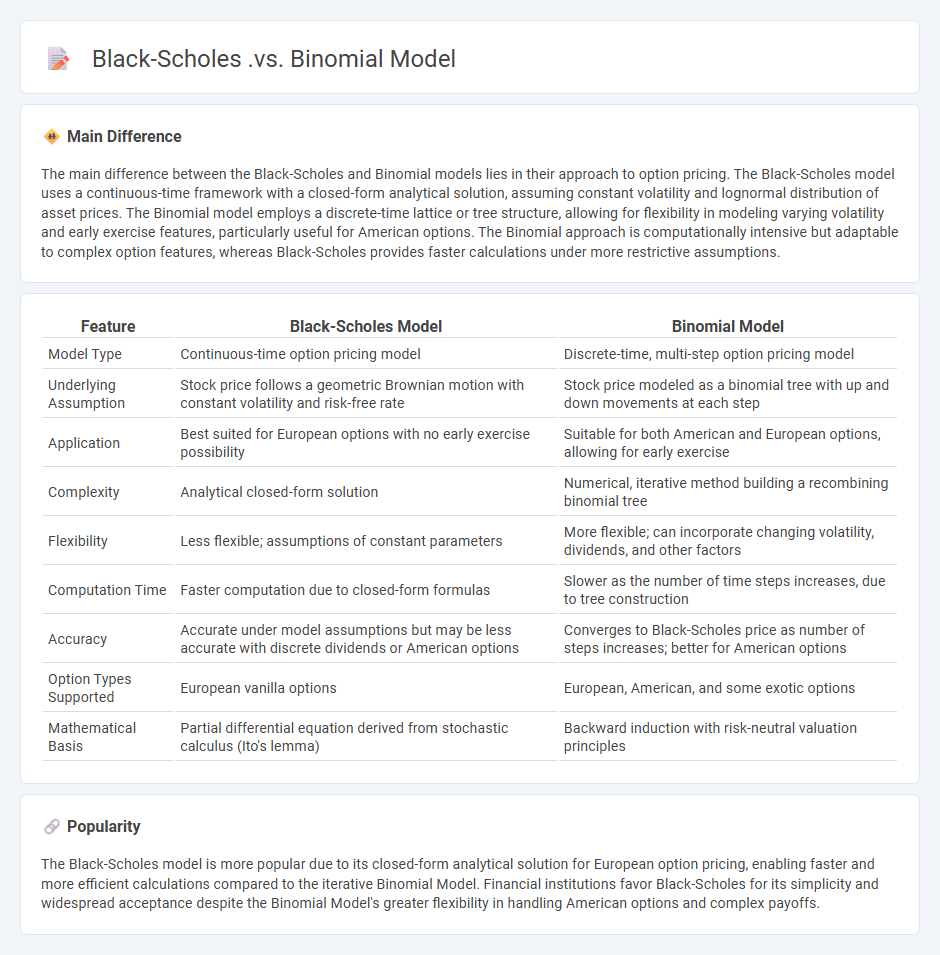
The main difference between the Black-Scholes and Binomial models lies in their approach to option pricing. The Black-Scholes model uses a continuous-time framework with a closed-form analytical solution, assuming constant volatility and lognormal distribution of asset prices. The Binomial model employs a discrete-time lattice or tree structure, allowing for flexibility in modeling varying volatility and early exercise features, particularly useful for American options. The Binomial approach is computationally intensive but adaptable to complex option features, whereas Black-Scholes provides faster calculations under more restrictive assumptions.
Connection
The Black-Scholes model is derived as the continuous-time limit of the Binomial Model when the number of time steps approaches infinity and the size of each step becomes infinitesimally small. Both models are used for option pricing, with the Binomial Model providing a discrete-time framework and the Black-Scholes offering a closed-form analytical solution under the assumptions of geometric Brownian motion. The connection ensures consistency between discrete-time numerical approximations and continuous-time theoretical pricing methods in financial derivatives valuation.
Comparison Table
| Feature | Black-Scholes Model | Binomial Model |
|---|---|---|
| Model Type | Continuous-time option pricing model | Discrete-time, multi-step option pricing model |
| Underlying Assumption | Stock price follows a geometric Brownian motion with constant volatility and risk-free rate | Stock price modeled as a binomial tree with up and down movements at each step |
| Application | Best suited for European options with no early exercise possibility | Suitable for both American and European options, allowing for early exercise |
| Complexity | Analytical closed-form solution | Numerical, iterative method building a recombining binomial tree |
| Flexibility | Less flexible; assumptions of constant parameters | More flexible; can incorporate changing volatility, dividends, and other factors |
| Computation Time | Faster computation due to closed-form formulas | Slower as the number of time steps increases, due to tree construction |
| Accuracy | Accurate under model assumptions but may be less accurate with discrete dividends or American options | Converges to Black-Scholes price as number of steps increases; better for American options |
| Option Types Supported | European vanilla options | European, American, and some exotic options |
| Mathematical Basis | Partial differential equation derived from stochastic calculus (Ito's lemma) | Backward induction with risk-neutral valuation principles |
Option Pricing
Option pricing models, such as the Black-Scholes-Merton framework, play a crucial role in determining the fair value of financial derivatives. These models incorporate variables like the underlying asset price, strike price, time to expiration, volatility, and risk-free interest rate. Accurate option pricing enables traders and investors to manage risk, optimize portfolios, and implement hedging strategies effectively. Market data and implied volatility remain essential inputs for refining pricing accuracy and estimating options' market behavior.
Continuous vs. Discrete Time
Continuous time finance models capture asset price movements with infinite precision, representing prices as functions defined for every instant, which allows for advanced tools like stochastic calculus and differential equations. Discrete time models approximate price changes at specific intervals, simplifying computations and fitting well with actual market data recorded in daily or monthly snapshots. Key continuous time frameworks include the Black-Scholes-Merton model for option pricing, while discrete models often employ binomial trees and autoregressive processes. The choice between continuous and discrete time impacts risk assessment, hedging strategies, and derivative pricing in quantitative finance.
Volatility Assumptions
Volatility assumptions play a critical role in financial modeling, impacting option pricing, risk management, and portfolio optimization. Traders and analysts often use historical volatility, implied volatility from options markets, and stochastic volatility models to estimate future price fluctuations. Accurate volatility estimates enhance the precision of derivative valuations under models like Black-Scholes and Heston, influencing hedging strategies and capital allocation. Market microstructure factors and macroeconomic events are key drivers that dynamically affect volatility assumptions in practice.
Hedging Strategies
Hedging strategies in finance involve using financial instruments like options, futures, and swaps to reduce exposure to market risks such as price fluctuations, interest rate changes, and currency volatility. Corporations and investors implement these tactics to protect asset values and stabilize cash flows. For example, oil companies might use futures contracts to lock in prices and mitigate the impact of volatile crude oil markets. Effective hedging enhances financial planning accuracy and supports long-term investment stability.
American vs. European Options
American options can be exercised at any time up to the expiration date, providing greater flexibility and potential for strategic trading. European options, in contrast, can only be exercised at maturity, often resulting in lower premiums and simpler pricing models. The Black-Scholes model is commonly used for European options valuation, while American options require more complex methods like binomial trees due to their early exercise feature. Understanding these differences is crucial for investors managing risk and optimizing their derivatives portfolio.
Source and External Links
Proof the Binomial Model Converges to Black-Scholes - The binomial options-pricing model converges precisely to the Black-Scholes model as the number of discrete time steps approaches infinity.
Binomial Model vs. Black Scholes - Strategic Investments - The binomial model offers greater flexibility for real-world modeling, especially for American options and projects with complex timing, while Black-Scholes is less adaptable due to its fixed, continuous-time framework.
Option Pricing Models (Black-Scholes & Binomial) - Hoadley.net - The binomial model can price American options accurately and serves as a discrete approximation to Black-Scholes, which is analytic and efficient for European options as a special limiting case.
FAQs
What is the Black-Scholes model?
The Black-Scholes model is a mathematical framework used to calculate the theoretical price of European-style options by modeling the dynamics of the underlying asset's price with geometric Brownian motion and applying partial differential equations.
What is the Binomial model?
The Binomial model is a mathematical framework used in finance to price options by simulating possible price paths of the underlying asset through discrete time steps, calculating option values backward from expiration to the present.
How does Black-Scholes differ from the Binomial model?
The Black-Scholes model provides a closed-form analytical solution for European option pricing assuming continuous time and constant volatility, while the Binomial model uses a discrete-time lattice framework to approximate option prices and can handle American options and varying conditions.
What assumptions are made in the Black-Scholes model?
The Black-Scholes model assumes constant risk-free interest rates, lognormal distribution of stock prices, continuous trading, no arbitrage opportunities, no dividends, frictionless markets without taxes or transaction costs, and constant volatility.
How does the Binomial model handle American options?
The Binomial model handles American options by evaluating the option's value at each node through backward induction, comparing the immediate exercise value with the expected hold value, and choosing the maximum to account for the early exercise feature.
Which model is more accurate for option pricing?
The Black-Scholes model is more accurate for European option pricing under the assumptions of constant volatility and no dividends, while the Binomial model offers greater flexibility and accuracy for American options and scenarios with changing conditions.
When should you use the Black-Scholes or Binomial model?
Use the Black-Scholes model for pricing European options with constant volatility and interest rates; use the Binomial model for American options, allowing early exercise, or when modeling variable volatility and interest rates.