Geometric mean return measures the compound growth rate of an investment over multiple periods, accurately reflecting the effect of volatility and compounding. Arithmetic mean return calculates the simple average of returns, often overestimating long-term performance by ignoring compounding effects. Explore the key differences and applications of geometric and arithmetic mean returns to enhance your investment analysis.
Main Difference
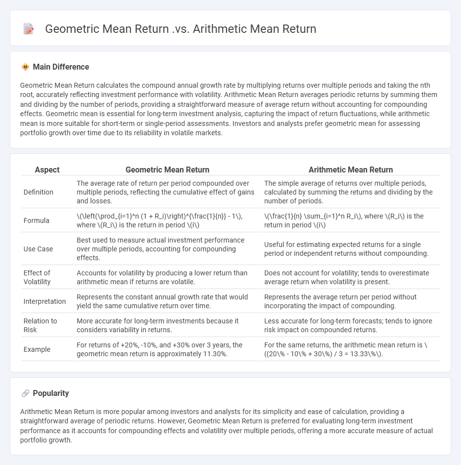
Geometric Mean Return calculates the compound annual growth rate by multiplying returns over multiple periods and taking the nth root, accurately reflecting investment performance with volatility. Arithmetic Mean Return averages periodic returns by summing them and dividing by the number of periods, providing a straightforward measure of average return without accounting for compounding effects. Geometric mean is essential for long-term investment analysis, capturing the impact of return fluctuations, while arithmetic mean is more suitable for short-term or single-period assessments. Investors and analysts prefer geometric mean for assessing portfolio growth over time due to its reliability in volatile markets.
Connection
Geometric mean return and arithmetic mean return are connected through the variability of investment returns, where the geometric mean accounts for compounding effects over time and typically falls below the arithmetic mean when returns are volatile. The arithmetic mean calculates the simple average of periodic returns, while the geometric mean provides a more accurate measure of the actual average growth rate by multiplying returns across periods. The difference between these means is influenced by the variance of returns and can be approximated using the formula: Geometric Mean Arithmetic Mean - (Variance/2).
Comparison Table
| Aspect | Geometric Mean Return | Arithmetic Mean Return |
|---|---|---|
| Definition | The average rate of return per period compounded over multiple periods, reflecting the cumulative effect of gains and losses. | The simple average of returns over multiple periods, calculated by summing the returns and dividing by the number of periods. |
| Formula | \(\left(\prod_{i=1}^n (1 + R_i)\right)^{\frac{1}{n}} - 1\), where \(R_i\) is the return in period \(i\) | \(\frac{1}{n} \sum_{i=1}^n R_i\), where \(R_i\) is the return in period \(i\) |
| Use Case | Best used to measure actual investment performance over multiple periods, accounting for compounding effects. | Useful for estimating expected returns for a single period or independent returns without compounding. |
| Effect of Volatility | Accounts for volatility by producing a lower return than arithmetic mean if returns are volatile. | Does not account for volatility; tends to overestimate average return when volatility is present. |
| Interpretation | Represents the constant annual growth rate that would yield the same cumulative return over time. | Represents the average return per period without incorporating the impact of compounding. |
| Relation to Risk | More accurate for long-term investments because it considers variability in returns. | Less accurate for long-term forecasts; tends to ignore risk impact on compounded returns. |
| Example | For returns of +20%, -10%, and +30% over 3 years, the geometric mean return is approximately 11.30%. | For the same returns, the arithmetic mean return is \((20\% - 10\% + 30\%) / 3 = 13.33\%\). |
Compounding Effect
The compounding effect in finance refers to the process where investment earnings generate additional earnings over time, creating exponential growth. This effect occurs when interest or returns are reinvested, allowing capital to grow at an increasing rate, as demonstrated by Albert Einstein's description of compounding as the "eighth wonder of the world." According to historical data, the S&P 500 has delivered an average annual return of approximately 10%, highlighting the power of compounding in long-term stock market investments. Understanding the compounding effect is essential for retirement planning, as even small contributions can accumulate significantly over decades.
Time-weighted Return
Time-weighted return (TWR) measures the compound growth rate of an investment portfolio, eliminating the influence of cash inflows and outflows. Widely used in finance, it enables accurate performance comparison across portfolios by isolating the effect of investment decisions from external cash movements. Calculated by segmenting the portfolio into sub-periods between cash flows and linking the returns geometrically, TWR reflects the true manager's skill. This metric is essential for evaluating mutual funds, hedge funds, and wealth management services with varying cash flow activity.
Volatility Impact
Volatility impact measures the degree of asset price fluctuations affecting investment risk and return profiles. High volatility increases the potential for significant gains or losses, influencing portfolio diversification and risk management strategies. Financial instruments like options and derivatives are directly sensitive to volatility changes, with metrics such as the VIX index quantifying market volatility levels. Understanding volatility impact is crucial for traders and fund managers to optimize asset allocation and hedge against market instability.
Average Periodic Return
Average periodic return represents the mean rate of return on an investment over a specific time interval, such as daily, monthly, or quarterly periods. It is calculated by summing all periodic returns and dividing by the number of periods, providing insight into investment performance consistency. This metric is fundamental for evaluating mutual funds, ETFs, or individual securities to assess their growth trends. Analysts use average periodic return alongside measures like standard deviation to gauge risk-adjusted returns effectively.
Performance Measurement
Performance measurement in finance evaluates the effectiveness of investment portfolios, funds, and financial strategies through metrics like return on investment (ROI), alpha, and Sharpe ratio. Accurate measurement involves comparing actual returns to benchmarks such as the S&P 500 or MSCI World Index. Risk-adjusted performance metrics consider volatility, using standard deviation and beta, to assess efficiency. Tools like performance attribution break down returns by asset class and sector to identify value drivers.
Source and External Links
Arithmetic Returns vs. Geometric Returns - Bogleheads.org - The geometric mean return accounts for compounding by taking the product of (1 + returns) raised to the power of 1/n minus one, and is always less than or equal to the arithmetic mean return, which is the simple average of returns, due to volatility effects.
Arithmetic Mean Vs Geometric Mean - Differences, Table, Examples - The arithmetic mean is the sum of values divided by their count, while the geometric mean is the nth root of the product of values; the geometric mean only applies to positive numbers and is typically less than the arithmetic mean for the same data set.
Arithmetic vs. Geometric Return | Definition & Calculation - Lesson - The arithmetic mean calculates the simple average of returns ignoring cumulative effects, while the geometric mean properly reflects compounding over time, giving a more accurate picture of actual investment performance especially when returns vary widely.
FAQs
What is a mean return in finance?
Mean return in finance is the average percentage gain or loss of an investment over a specified period, calculated by summing all periodic returns and dividing by the number of periods.
What is the arithmetic mean return?
The arithmetic mean return is the sum of individual returns divided by the number of periods, representing the average periodic return over a specific time frame.
What is the geometric mean return?
The geometric mean return is the average compound rate of return per period on an investment, calculated as the nth root of the product of (1 + each period's return) minus 1, reflecting the cumulative effect of returns over multiple periods.
How is arithmetic mean return calculated?
The arithmetic mean return is calculated by summing all individual returns over a period and dividing by the total number of returns.
How is geometric mean return calculated?
Geometric mean return is calculated by taking the nth root of the product of (1 plus each periodic return) over n periods, then subtracting 1: Geometric Mean Return = [((1 + R_i))^(1/n)] - 1, where R_i represents each individual periodic return and n is the total number of periods.
What is the key difference between arithmetic and geometric mean returns?
The key difference is that the arithmetic mean return calculates the simple average of periodic returns, assuming independent periods, while the geometric mean return accounts for compounding by calculating the nth root of the product of (1 + returns), reflecting the actual cumulative growth rate over multiple periods.
When should you use geometric mean return over arithmetic mean return?
Use geometric mean return to measure average investment performance over multiple periods when accounting for compounding effects and variable returns; use arithmetic mean return for estimating expected return in a single-period or independent-period context without compounding.