The Gordon Growth Model estimates a stock's intrinsic value assuming a constant dividend growth rate, providing simplicity for stable companies with predictable dividends. The Two-Stage Dividend Discount Model accommodates varying growth rates by splitting dividend growth into two phases, capturing firms experiencing accelerated early growth followed by stable maturity. Explore these models further to determine which dividend valuation approach suits your investment analysis.
Main Difference
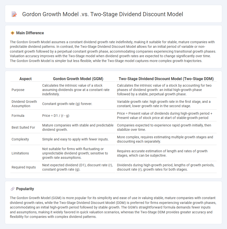
The Gordon Growth Model assumes a constant dividend growth rate indefinitely, making it suitable for stable, mature companies with predictable dividend patterns. In contrast, the Two-Stage Dividend Discount Model allows for an initial period of variable or non-constant growth followed by a perpetual constant growth phase, accommodating companies experiencing transitional growth phases. Valuation accuracy improves with the Two-Stage model when dividend growth rates are expected to change significantly over time. The Gordon Growth Model is simpler but less flexible, while the Two-Stage model captures more complex growth trajectories.
Connection
The Gordon Growth Model (GGM) is a simplified version of the Two-Stage Dividend Discount Model (DDM), focusing on a constant growth rate of dividends indefinitely. The Two-Stage DDM expands on this by incorporating an initial period of non-constant or high growth followed by a stable, perpetual growth phase, reflecting more realistic dividend patterns. Both models use discounted dividends to estimate intrinsic stock value, linking their fundamental valuation approach through dividend projections and discount rates.
Comparison Table
| Aspect | Gordon Growth Model (GGM) | Two-Stage Dividend Discount Model (Two-Stage DDM) |
|---|---|---|
| Purpose | Calculates the intrinsic value of a stock assuming dividends grow at a constant rate indefinitely. | Calculates the intrinsic value of a stock by accounting for two phases of dividend growth: an initial high-growth phase followed by a stable, perpetual growth phase. |
| Dividend Growth Assumption | Constant growth rate (g) forever. | Variable growth rate: high growth rate in the first stage, and a constant, lower growth rate in the second stage. |
| Formula | Price = D1 / (r - g) | Price = Present value of dividends during high-growth period + Present value of stock price at start of stable-growth period |
| Best Suited For | Mature companies with stable and predictable dividend growth. | Companies expected to experience rapid growth initially, then stabilize over time. |
| Complexity | Simple and easy to apply with fewer inputs. | More complex, requires estimating multiple growth stages and discounting each separately. |
| Limitations | Not suitable for firms with fluctuating or unpredictable dividend growth; sensitive to growth rate assumptions. | Requires accurate estimation of length and rates of growth stages, which can be subjective. |
| Required Inputs | Next expected dividend (D1), discount rate (r), constant growth rate (g). | Dividends during high-growth period, lengths of growth periods, discount rate (r), growth rates for both stages. |
Constant Growth Assumption
Constant Growth Assumption in finance refers to the premise that a company's dividends will increase at a consistent, steady rate indefinitely. This assumption underpins the Gordon Growth Model, a commonly used method to value stocks by discounting expected future dividends. Analysts often apply this model to mature firms with stable earnings and dividend histories. The key input, the constant growth rate, typically aligns closely with the historical dividend growth rate or long-term GDP growth projections.
Multiple Growth Phases
Multiple growth phases in finance refer to distinct periods within a company's lifecycle characterized by varying rates of revenue and profit expansion. Early stages often exhibit rapid growth fueled by innovation and market penetration, followed by maturity phases with stabilized earnings and slower growth rates. Investors analyze these phases to forecast cash flows, assess risk, and determine valuation metrics such as price-to-earnings (P/E) ratios and discounted cash flow (DCF) models. Understanding multiple growth phases enables more accurate financial modeling and strategic decision-making for capital allocation.
Terminal Value Calculation
Terminal value calculation in finance estimates the present value of all future cash flows beyond a forecast period in discounted cash flow (DCF) analysis. Common methods include the perpetuity growth model, which assumes a constant growth rate in cash flows, and the exit multiple approach, based on industry comparables. Accurate terminal value estimation is critical as it often represents over 50% of a company's total valuation. Key inputs involve the discount rate, typically the weighted average cost of capital (WACC), and a sustainable growth rate aligned with long-term economic projections.
Applicability to Mature vs. High-Growth Firms
Mature firms typically exhibit stable cash flows and established market positions, which influence their capital structure decisions and dividend policies differently than high-growth firms. High-growth firms prioritize reinvestment of earnings to fuel expansion, often relying more on equity financing due to limited retained earnings and higher risk profiles. The cost of capital varies between these firms, with mature companies often benefiting from lower equity costs and easier access to debt markets. Understanding these differences is crucial for tailoring financial strategies that optimize firm value and support long-term growth objectives.
Sensitivity to Dividend Estimates
Sensitivity to dividend estimates plays a critical role in equity valuation models, impacting stock price predictions and investment decisions. Small variations in expected dividend growth rates or payout amounts can significantly alter discounted cash flow (DCF) valuations and dividend discount models (DDM). Financial analysts utilize sensitivity analysis techniques to assess how changes in dividend assumptions affect intrinsic values, helping to manage risk and inform portfolio strategies. Accurate dividend forecasting is essential for optimizing asset allocation and maximizing shareholder returns in dynamic market environments.
Source and External Links
11.2 Dividend Discount Models (DDMs) - Principles of Finance - The Gordon Growth Model assumes a constant dividend growth rate indefinitely, while the Two-Stage Dividend Discount Model accounts for two phases: an initial period of higher growth followed by a stable, lower growth rate, making it more realistic for valuing mature companies.
The Two-Stage Dividend Discount Model - The two-stage model improves on the Gordon Growth Model by incorporating a sharp transition between two growth rates (initial high and subsequent stable), but it still assumes sudden changes and constant growth rates within each stage.
The Three-Stage Dividend Discount Model - The Gordon Growth Model forms the basis for all DDMs but is the simplest and least accurate due to its constant growth assumption, while the two-stage model allows changing dividend growth rates with a sharp transition, and the three-stage model allows gradual changes for even more nuanced valuation.
FAQs
What is the Gordon Growth Model?
The Gordon Growth Model is a valuation method that calculates the intrinsic value of a stock by dividing the expected annual dividend per share by the difference between the required rate of return and the constant dividend growth rate.
What is the Two-Stage Dividend Discount Model?
The Two-Stage Dividend Discount Model values a stock by estimating dividends with an initial high growth rate for a specific period, followed by a stable, lower growth rate indefinitely.
How does the Gordon Growth Model work?
The Gordon Growth Model calculates a stock's intrinsic value by dividing the expected annual dividend per share by the difference between the required rate of return and the constant dividend growth rate.
How does the Two-Stage Dividend Discount Model work?
The Two-Stage Dividend Discount Model values a stock by first estimating dividends growing at a high, non-constant rate for an initial period, then applying a stable, constant growth rate thereafter, discounting all projected dividends back to present value using the required rate of return.
What are the key assumptions of each model?
Key assumptions of the Classical Linear Regression Model include linearity between dependent and independent variables, independence of errors, homoscedasticity (constant variance of errors), no perfect multicollinearity among predictors, and normally distributed errors. The Assumptions of the Probit Model include a latent continuous variable underlying the binary outcome, normally distributed error terms, independence across observations, and correct specification of the link function. The Logistic Regression Model assumes a logistic distribution of errors, a linear relationship between predictors and the log-odds of the outcome, independence of observations, and absence of multicollinearity among predictors. The Time Series ARIMA Model assumes stationarity after differencing, linearity, independence and normality of residuals, and that the model order (p, d, q) correctly captures the data's autocorrelation and differencing structure.
When should you use the Gordon Growth Model vs the Two-Stage Dividend Discount Model?
Use the Gordon Growth Model for valuing stocks with dividends expected to grow at a constant, stable rate indefinitely; apply the Two-Stage Dividend Discount Model when dividends are expected to grow at different rates during an initial phase before stabilizing into a constant growth phase.
What are the limitations of both models?
Model A's limitations include high computational cost and overfitting on small datasets; Model B struggles with interpretability and lower accuracy in complex scenarios.