Euler Method offers a straightforward, first-order numerical approach for solving ordinary differential equations, ideal for simple problems with limited accuracy requirements. In contrast, Runge-Kutta Methods provide higher-order solutions by evaluating intermediate points, significantly improving precision and stability in complex systems. Explore detailed comparisons to determine the optimal method for your computational needs.
Main Difference
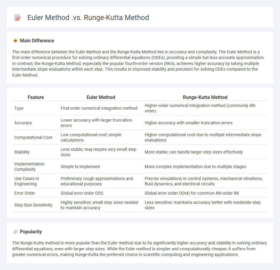
The main difference between the Euler Method and the Runge-Kutta Method lies in accuracy and complexity. The Euler Method is a first-order numerical procedure for solving ordinary differential equations (ODEs), providing a simple but less accurate approximation. In contrast, the Runge-Kutta Method, especially the popular fourth-order version (RK4), achieves higher accuracy by taking multiple intermediate slope evaluations within each step. This results in improved stability and precision for solving ODEs compared to the Euler Method.
Connection
Euler Method serves as the foundational numerical technique for solving ordinary differential equations, using a first-order approximation of derivatives. Runge-Kutta Method builds upon Euler's approach by incorporating multiple intermediate slopes within each step, achieving higher-order accuracy and improved stability. Both methods discretize continuous problems but differ significantly in precision and computational complexity.
Comparison Table
| Feature | Euler Method | Runge-Kutta Method |
|---|---|---|
| Type | First-order numerical integration method | Higher-order numerical integration method (commonly 4th order) |
| Accuracy | Lower accuracy with larger truncation errors | Higher accuracy with smaller truncation errors |
| Computational Cost | Low computational cost; simple calculations | Higher computational cost due to multiple intermediate slope evaluations |
| Stability | Less stable; may require very small step sizes | More stable; can handle larger step sizes effectively |
| Implementation Complexity | Simple to implement | More complex implementation due to multiple stages |
| Use Cases in Engineering | Preliminary rough approximations and educational purposes | Precise simulations in control systems, mechanical vibrations, fluid dynamics, and electrical circuits |
| Error Order | Global error order O(h) | Global error order O(h4) for common 4th-order RK |
| Step Size Sensitivity | Highly sensitive; small step sizes needed to maintain accuracy | Less sensitive; maintains accuracy better with moderate step sizes |
Numerical Integration
Numerical integration methods such as the trapezoidal rule, Simpson's rule, and Gaussian quadrature are essential tools in engineering for approximating definite integrals when analytical solutions are infeasible. These techniques are widely applied in fields like civil, mechanical, and electrical engineering to analyze stress distributions, heat transfer, and signal processing. Advanced algorithms leverage adaptive quadrature to increase accuracy while minimizing computational cost. Software packages like MATLAB and ANSYS commonly implement these numerical integration methods for engineering simulations and finite element analysis.
Local Truncation Error
Local truncation error measures the discrepancy introduced in a single step of a numerical method when solving differential equations. It quantifies the difference between the exact and numerical solution over one iteration, impacting the overall accuracy of engineering simulations. Precise evaluation of local truncation error informs the selection of step size and numerical schemes in finite element analysis and computational fluid dynamics. Minimizing this error enhances the reliability of predictions in structural modeling, heat transfer, and system dynamics.
Stability Analysis
Stability analysis in engineering evaluates the ability of structures or systems to maintain equilibrium under various loads or disturbances. It involves mathematical modeling and computational methods to predict potential failure modes such as buckling, dynamic instability, or resonance. Common applications include civil engineering structures like bridges and buildings, mechanical systems, and control systems in aerospace engineering. Techniques like eigenvalue analysis, Lyapunov methods, and finite element analysis are extensively employed to ensure safety and reliability.
Computational Complexity
Computational complexity in engineering quantifies the resources required for algorithms to solve practical problems, focusing on time and space efficiency. It assists engineers in selecting optimal algorithms that balance performance and computational cost when designing systems and simulations. Analyzing complexity classes such as P, NP, and NP-hard informs engineers about problem tractability and feasibility in real-world applications. This knowledge drives advancements in areas like signal processing, control systems, and data analysis by enabling efficient computation under resource constraints.
Differential Equations Modeling
Differential equations are fundamental in engineering for modeling dynamic systems and describing how physical quantities change over time. They are extensively used in fields such as mechanical engineering for vibration analysis, electrical engineering for circuit design, and chemical engineering for reaction kinetics. Engineers apply techniques like Laplace transforms and numerical methods to solve ordinary and partial differential equations, enabling precise system predictions and control. The practical implementation of these models supports optimization, stability assessment, and real-time monitoring in engineering projects.
Source and External Links
Comparative study of Euler's method and Runge-Kutta method to solve an ordinary differential equation through a computational approach - The Runge-Kutta method generally provides better accuracy than Euler's method for solving differential equations, especially with small step sizes, while Euler's method is simpler but less accurate for larger steps.
Runge-Kutta methods - Wikipedia - Runge-Kutta methods are a family of iterative techniques that extend Euler's method by improving stability and accuracy, with explicit methods like RK4 being more accurate than Euler's first-order method.
Why Runge-Kutta is SO Much Better Than Euler's Method #somepi - Runge-Kutta methods, especially RK4, are widely preferred over Euler's method because they drastically reduce error and increase accuracy by averaging multiple slope estimates, while Euler's method can become inaccurate quickly as time progresses.
FAQs
What is the Euler method?
The Euler method is a first-order numerical technique for solving ordinary differential equations by approximating solutions using tangent line slopes at discrete points.
What is the Runge-Kutta method?
The Runge-Kutta method is a numerical technique for solving ordinary differential equations by approximating solutions through weighted averages of slopes at multiple points within each integration step.
How does Euler method differ from Runge-Kutta method?
Euler method uses a single slope estimate per step for numerical integration, while Runge-Kutta method employs multiple slope evaluations within each step to achieve higher accuracy.
When should you use Euler method over Runge-Kutta?
Use the Euler method over Runge-Kutta for solving ordinary differential equations when computational simplicity and speed are prioritized, and problem accuracy or stability requirements are low.
What are the advantages of the Runge-Kutta method?
The Runge-Kutta method offers high accuracy, simplicity in implementation, and strong stability for solving ordinary differential equations without requiring higher-order derivatives.
Which method is more accurate and why?
The method using deep learning with convolutional neural networks (CNNs) is more accurate due to its ability to automatically extract hierarchical features and adapt to complex data patterns.
What are the limitations of Euler and Runge-Kutta methods?
Euler method is limited by low accuracy and numerical instability for stiff or highly nonlinear problems. Runge-Kutta methods, while more accurate, face challenges with computational cost, complexity for higher orders, and potential instability in stiff equations without implicit formulations.