Lumped parameter models simplify complex systems by representing them with discrete components, ideal for analyzing systems where spatial variations are negligible. Distributed parameter models capture spatially varying properties using partial differential equations, providing detailed insights into systems with significant spatial heterogeneity. Explore the strengths and applications of each modeling approach to enhance your system analysis capabilities.
Main Difference
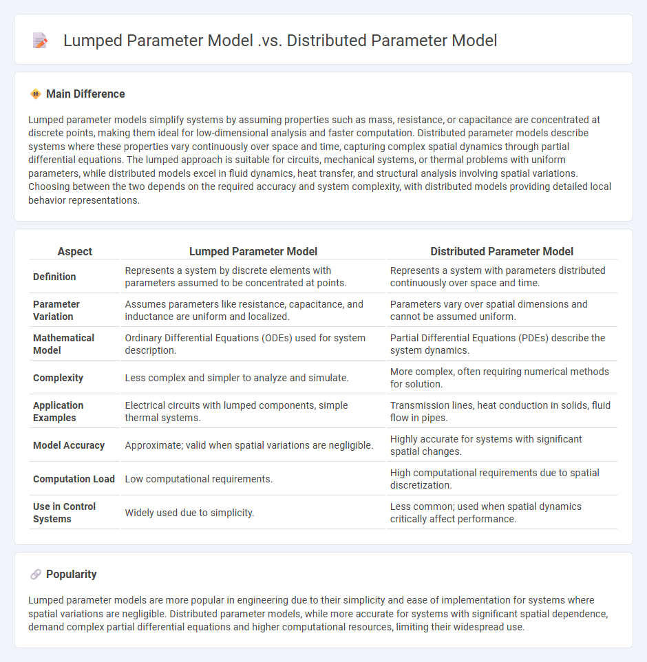
Lumped parameter models simplify systems by assuming properties such as mass, resistance, or capacitance are concentrated at discrete points, making them ideal for low-dimensional analysis and faster computation. Distributed parameter models describe systems where these properties vary continuously over space and time, capturing complex spatial dynamics through partial differential equations. The lumped approach is suitable for circuits, mechanical systems, or thermal problems with uniform parameters, while distributed models excel in fluid dynamics, heat transfer, and structural analysis involving spatial variations. Choosing between the two depends on the required accuracy and system complexity, with distributed models providing detailed local behavior representations.
Connection
Lumped parameter models approximate system behavior using discrete elements with uniform properties, while distributed parameter models represent spatially continuous variations in parameters. The connection lies in the lumped model being a simplified, finite-dimensional abstraction of the infinite-dimensional distributed model obtained through spatial discretization methods such as finite element or finite difference techniques. This derivation maintains key physical characteristics while reducing complexity for easier analysis and control design.
Comparison Table
| Aspect | Lumped Parameter Model | Distributed Parameter Model |
|---|---|---|
| Definition | Represents a system by discrete elements with parameters assumed to be concentrated at points. | Represents a system with parameters distributed continuously over space and time. |
| Parameter Variation | Assumes parameters like resistance, capacitance, and inductance are uniform and localized. | Parameters vary over spatial dimensions and cannot be assumed uniform. |
| Mathematical Model | Ordinary Differential Equations (ODEs) used for system description. | Partial Differential Equations (PDEs) describe the system dynamics. |
| Complexity | Less complex and simpler to analyze and simulate. | More complex, often requiring numerical methods for solution. |
| Application Examples | Electrical circuits with lumped components, simple thermal systems. | Transmission lines, heat conduction in solids, fluid flow in pipes. |
| Model Accuracy | Approximate; valid when spatial variations are negligible. | Highly accurate for systems with significant spatial changes. |
| Computation Load | Low computational requirements. | High computational requirements due to spatial discretization. |
| Use in Control Systems | Widely used due to simplicity. | Less common; used when spatial dynamics critically affect performance. |
Spatial Variation
Spatial variation in engineering refers to the differences in material properties, geometric features, or environmental conditions observed across a physical space within a structure or system. It significantly impacts the performance, durability, and safety of engineering components, influencing factors such as stress distribution, thermal conductivity, and fluid flow. Advanced simulation tools and mapping techniques enable engineers to accurately model and predict spatial variations for optimized design and maintenance strategies. Understanding spatial variation is essential in fields like civil engineering, aerospace, and manufacturing to enhance structural integrity and functionality.
Model Complexity
Model complexity in engineering quantifies the intricacy of mathematical models used to simulate physical systems, often measured by the number of parameters, variables, and equations involved. High model complexity can improve accuracy but increases computational cost and challenges in interpretation and validation. Techniques such as dimensionality reduction, surrogate modeling, and sensitivity analysis help manage complexity while maintaining model fidelity. In fields like structural engineering and control systems, balancing model complexity is crucial for effective design and real-time application.
Differential Equations
Differential equations serve as foundational tools in engineering for modeling dynamic systems and describing relationships involving rates of change. They are extensively applied in fields such as mechanical, electrical, civil, and chemical engineering to analyze vibrations, heat transfer, fluid flow, and control systems. Techniques like separation of variables, Laplace transforms, and numerical methods enable engineers to solve ordinary and partial differential equations effectively. Mastery of differential equations enhances the design, optimization, and prediction capabilities critical to engineering innovations and problem-solving.
Application Domains
Engineering applications span diverse domains including civil, mechanical, electrical, and software engineering, each leveraging specialized tools and methodologies. Structural analysis in civil engineering ensures the safety and durability of buildings and infrastructure, utilizing finite element modeling and material science innovations. Mechanical engineering focuses on designing and manufacturing machinery, engines, and automated systems, integrating principles of thermodynamics and fluid mechanics. Electrical engineering encompasses power generation, control systems, and electronics, driving advancements in renewable energy and communication technologies.
Computational Requirements
Computational requirements in engineering involve the necessary processing power, memory capacity, and software tools essential for modeling, simulation, and data analysis. High-performance computing (HPC) platforms are often utilized to handle complex finite element analysis (FEA), computational fluid dynamics (CFD), and structural simulations. Efficient algorithms and parallel processing techniques enhance computational efficiency, enabling engineers to solve large-scale problems with precision. Cloud computing resources such as Amazon Web Services (AWS) and Microsoft Azure also support scalable engineering computations.
Source and External Links
How to understand Lumped-parameter and Distribution ... - UIY - A lumped parameter model assumes circuit components are much smaller than the wavelength and parameters like resistance or capacitance are concentrated at points, while a distributed parameter model considers the circuit size comparable to the wavelength with parameters distributed along the circuit, typical in high-frequency transmission lines.
Lumped Circuit Analysis Vs Distributed Analysis - Rahsoft - Lumped parameter analysis is valid for low frequencies where circuit size is much smaller than the signal wavelength, treating components as ideal and concentrated, whereas distributed parameter analysis applies at high frequencies where wavelength and component sizes are comparable, requiring accounting for parameter distribution and signal propagation effects.
The Difference Between Lumped and Distributed Elements in Microwave Circuits - Lumped elements are described by ordinary differential equations with voltages and currents as functions of time at singular points and no spatial variation, while distributed elements, such as transmission lines beyond a certain length, require partial differential equations as parameters vary along their length.
FAQs
What is a lumped parameter model?
A lumped parameter model represents a physical system by aggregating spatially distributed properties into discrete, simplified elements characterized by parameters such as resistance, capacitance, and inductance.
What is a distributed parameter model?
A distributed parameter model describes systems where state variables depend on spatial coordinates and time, typically represented by partial differential equations.
How do lumped and distributed parameter models differ?
Lumped parameter models assume system properties like mass, resistance, or capacitance are concentrated at discrete points, simplifying analysis into algebraic equations. Distributed parameter models represent properties continuously distributed over space, requiring partial differential equations to capture spatial variations accurately.
When should you use a lumped parameter model?
Use a lumped parameter model when system variables can be approximated as uniform throughout spatial dimensions, enabling simplified analysis of dynamic behavior without detailed spatial resolution.
What are examples of distributed parameter systems?
Examples of distributed parameter systems include heat conduction in a metal rod, fluid flow in pipelines, flexible beams undergoing vibration, and chemical concentration changes in reaction-diffusion processes.
What are the advantages of lumped parameter models?
Lumped parameter models offer computational efficiency, simplified analysis, reduced model complexity, and easier parameter estimation, enabling faster simulation and design in engineering systems.
Why are distributed parameter models important in engineering?
Distributed parameter models are important in engineering because they accurately describe systems with spatially varying properties, enabling precise analysis and control of processes like heat transfer, fluid flow, and structural dynamics.