The Black-Scholes Model offers a continuous-time framework for valuing European options, relying on assumptions such as constant volatility and lognormal distribution of asset prices. In contrast, the Binomial Options Model employs a discrete-time lattice approach, allowing for flexible modeling of American options with varying exercise opportunities and dividend adjustments. Explore the nuances and practical applications of both models to enhance your options pricing strategies.
Main Difference
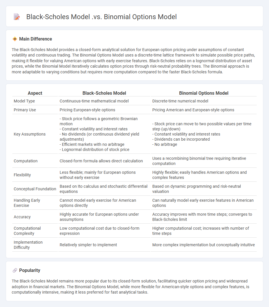
The Black-Scholes Model provides a closed-form analytical solution for European option pricing under assumptions of constant volatility and continuous trading. The Binomial Options Model uses a discrete-time lattice framework to simulate possible price paths, making it flexible for valuing American options with early exercise features. Black-Scholes relies on a lognormal distribution of asset prices, while the Binomial Model iteratively calculates option prices through risk-neutral probability trees. The Binomial approach is more adaptable to varying conditions but requires more computation compared to the faster Black-Scholes formula.
Connection
The Black-Scholes model and Binomial Options Pricing model are connected through their fundamental approach to option valuation based on replicating portfolios and risk-neutral valuation. The Binomial model provides a discrete-time framework that converges to the continuous-time Black-Scholes model as the number of time steps increases. Both models rely on assumptions about market efficiency, no arbitrage, and lognormal price distributions to estimate option prices accurately.
Comparison Table
| Aspect | Black-Scholes Model | Binomial Options Model |
|---|---|---|
| Model Type | Continuous-time mathematical model | Discrete-time numerical model |
| Primary Use | Pricing European-style options | Pricing American and European-style options |
| Key Assumptions |
- Stock price follows a geometric Brownian motion - Constant volatility and interest rates - No dividends (or continuous dividend yield adjustments) - Efficient markets with no arbitrage - Lognormal distribution of stock price |
- Stock price can move to two possible values per time step (up/down) - Constant volatility and interest rates - Dividends can be incorporated - No arbitrage |
| Computation | Closed-form formula allows direct calculation | Uses a recombining binomial tree requiring iterative computation |
| Flexibility | Less flexible; mainly for European options without early exercise | Highly flexible; easily handles American options and complex features |
| Conceptual Foundation | Based on Ito calculus and stochastic differential equations | Based on dynamic programming and risk-neutral valuation |
| Handling Early Exercise | Cannot model early exercise for American options directly | Can naturally model early exercise features in American options |
| Accuracy | Highly accurate for European options under assumptions | Accuracy improves with more time steps; converges to Black-Scholes limit |
| Computational Complexity | Low computational cost due to closed-form expression | Higher computational cost; increases with number of time steps |
| Implementation Difficulty | Relatively simpler to implement | More complex implementation but conceptually intuitive |
Continuous vs. Discrete Time
Continuous time models in finance use differential equations to represent asset price movements, assuming prices change at every instant, which aligns with the Black-Scholes option pricing framework. Discrete time models operate on fixed intervals, such as daily or quarterly returns, commonly applied in portfolio optimization and time series analysis like GARCH models. Continuous frameworks are preferred for derivative pricing due to their analytical tractability, while discrete models are favored for empirical financial data handling and risk management. The choice between continuous and discrete time modeling affects the estimation of volatility, risk measures, and the calibration of financial instruments.
Mathematical Complexity
Mathematical complexity in finance involves modeling intricate systems such as derivative pricing, risk assessment, and portfolio optimization using advanced methods like stochastic calculus, partial differential equations, and Monte Carlo simulations. Quantitative finance leverages complex algorithms to analyze market behaviors, predict asset price movements, and manage financial risks effectively. High-frequency trading platforms depend on real-time data processing and algorithmic strategies driven by complex mathematical frameworks. The integration of machine learning with traditional mathematical techniques further enhances predictive accuracy and financial decision-making.
Flexibility in Inputs
Flexibility in inputs within finance refers to the ability of financial models and systems to accommodate diverse data sources such as varying interest rates, fluctuating market indices, and multiple currency denominations. This adaptability enhances risk assessment accuracy and supports dynamic portfolio optimization under changing economic conditions. Ensuring input flexibility also improves the integration of alternative data, like social media sentiment and real-time transaction flows, which enrich predictive analytics. Financial institutions leveraging flexible input frameworks can respond more effectively to market volatility and regulatory changes.
Volatility Assumptions
Volatility assumptions play a crucial role in financial modeling, particularly in the pricing of options and risk management. These assumptions often rely on historical volatility data or implied volatility derived from market prices of derivatives. Accurate volatility estimation affects the calculation of Value at Risk (VaR) and the performance of trading strategies. Market participants frequently use models like GARCH or stochastic volatility models to capture changing market conditions.
American vs. European Options
American options can be exercised at any time before expiration, offering greater flexibility to traders in volatile markets. European options allow exercise only at expiration, often resulting in simpler valuation models like the Black-Scholes formula. In practice, American options are more common for equities, while European options dominate in index trading and certain currency derivatives. The choice influences pricing, hedging strategies, and risk management within financial portfolios.
Source and External Links
Option Pricing Models (Black-Scholes & Binomial) - Hoadley.net - The binomial model uses a computational, discrete approach to solve the same option pricing problem that the Black-Scholes model solves analytically; as the number of binomial steps increases, the binomial model converges to the Black-Scholes formula, making Black-Scholes a continuous limit of the binomial model, with binomial being better for American options due to its checking of early exercise opportunities.
Binomial Model vs. Black Scholes - Strategic Investments - The binomial model is more flexible and suitable for real option analysis, allowing varying time steps and decision tree structures not possible in Black-Scholes, which assumes fixed time development and cannot handle non-standard event trees, making binomial better for complex, less precise input variable environments.
Comparison: Binomial model and Black Scholes model - AIMS Press - The binomial model is a simple, discrete statistical method aligned with solving stochastic differential equations, while Black-Scholes requires continuous solutions; the binomial method matches Black-Scholes for European options and allows calibration through parameters ensuring recombining trees, reinforcing the conceptual link between the two methods.
FAQs
What is the Black-Scholes model?
The Black-Scholes model is a mathematical framework for pricing European-style options by calculating the theoretical value based on factors like the underlying asset price, strike price, time to expiration, risk-free interest rate, and asset volatility.
What is the Binomial Options model?
The Binomial Options model is a mathematical framework used to price options by modeling possible future asset prices through a discrete-time binomial tree, allowing calculation of option values via backward induction.
How do Black-Scholes and Binomial models differ?
The Black-Scholes model uses a continuous-time framework with closed-form solutions assuming constant volatility and risk-free rates, while the Binomial model employs a discrete-time lattice approach allowing for more flexible assumptions and easy handling of American options.
What are the assumptions of the Black-Scholes model?
The Black-Scholes model assumes a frictionless market, constant risk-free interest rate, constant volatility, lognormal distribution of stock prices, no dividends during the option's life, continuous trading, and no arbitrage opportunities.
What are the advantages of the Binomial Options model?
The Binomial Options model offers advantages such as simplicity, flexibility in handling various option types, accuracy through multi-step lattices, and suitability for valuing American options with early exercise features.
When should you use the Binomial model over Black-Scholes?
Use the Binomial model over Black-Scholes when modeling American options, incorporating discrete dividends, or requiring flexible, step-by-step pricing for path-dependent or early-exercise features.
Which model is more accurate for American options?
The Binomial model is more accurate for American options due to its ability to handle early exercise features.